PCA analysis
Installation
pip install Bio
pip install sklearn
Dependencies
R
install.packages("ade4")
Datasets
Download Rice 3K RG 404k CoreSNP Dataset, all chromosomes
cd data
wget https://s3.amazonaws.com/3kricegenome/snpseek-dl/3krg-base-filt-core-v0.7/core_v0.7.bed.gz
wget https://s3.amazonaws.com/3kricegenome/snpseek-dl/3krg-base-filt-core-v0.7/core_v0.7.bim.gz
wget https://s3.amazonaws.com/3kricegenome/snpseek-dl/3krg-base-filt-core-v0.7/core_v0.7.fam.gz

gunzip core_v0.7.bed.gz
gunzip core_v0.7.bim.gz
gunzip core_v0.7.fam.gz
Download information for a subset of these accession
wget https://raw.githubusercontent.com/SantosJGND/Galaxy_KDE_classifier/v1.2/Downstream_functions/Analyses_Jsubtrop_self_KDE/Order_core.txt
grep -v "COUNTRY" Order_core.txt | cut -f 2 > sample.txt
Workflow
Convert to vcf using plink
plink --bfile core_v0.7 --recode vcf-iid --keep-fam sample.txt --out core_v0.7
Adjust some missing value on vcf file
sed -i 's=GT=GT:AD:DP=' core_v0.7.vcf
sed -i 's=0/0=0/0:20,0:20=g' core_v0.7.vcf
sed -i 's=0/1=0/1:10,10:20=g' core_v0.7.vcf
sed -i 's=1/1=1/1:0,20:20=g' core_v0.7.vcf
sed -i 's=\.\/\.=\.\/\.:\.,\.:\.=g' core_v0.7.vcf
The first step of the Chromosome painting is to perform a PCA analysis on the vcf file to cluster the alleles and the accession.
Create a folder in which the analysis will be performed and run the following command line:
mkdir PCA
bin/vcf2struct.1.0.py --vcf data/core_v0.7.vcf --names data/sample.txt --type FACTORIAL --prefix PCA/Analysis --nAxes 6 --mulType coa
The last command line run the factorial analysis (–type FACTORIAL option). During this analysis the vcf file is recoded as followed : For each allele at each variants site two markers were generated; One marker for the presence of the allele (0/1 coded) and one for the absence of the allele (0/1 coded).

Only alleles present or absent in part (not all) of selected accessions were included in the final matrix file named PCA/Analysis_matrix_4_PCA.tab in this example. An additional column named “GROUP” can be identified. This column is filled with “UN” value if no –group argument is passed. We will explain later this argument.
The factorial analysis (here a COA, –mulType option) was performed on the transposed matrix using R (The R script is generated by the script and can be found here: PCA/Analysis_multivariate.R). R warning messages and command lines are recorded in the file named Analysis_multivariate.Rout. Graphical outputs of the analysis were draw and for example accessions and alleles can be projected along axis in the following picture.
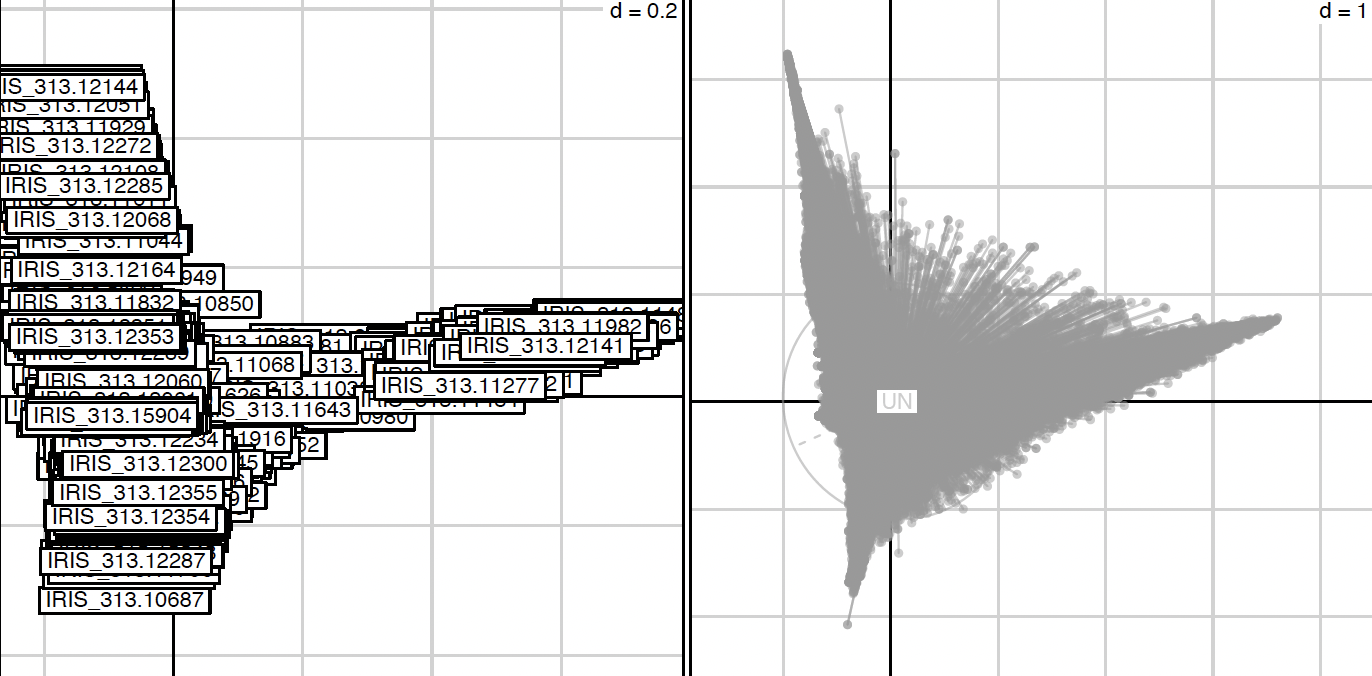
Correspond to the file : PCA/Analysis_axis_1_vs_2.pdf
In this example the left graph represent accessions projected along axis 1 and 2 and the right represent the allele projected along synthetic axis. A graphical representation is performed for each axis combinations and each file is named according to the following nomenclature *prefix + _axis_X_vs_Y.pdf*. Several pdf for accessions along axis only is also generated and are named according to the following nomenclature *prefix + _axis_X_vs_Y_accessions.pdf*.
Individual and variables coordinates for the selected 6 first axis (–nAxes option) are recorded in files named PCA/Analysis_individuals_coordinates.tab and PCA/Analysis_variables_coordinates.tab respectively. A third file named PCA/Analysis_variables_coordinates_scaled.tab containing allele scaled coordinates (columns centered and reduced) along synthetic axis is generated.
sort -k 2n,2 PCA/Analysis_individuals_coordinates.tab | cut -f 1 -d " " | tail -10 | sed 's:\"::g' | sed  's=\.=-=' | sed "s:$:\tg1:" > group1.txt
sort -k 3n,3 PCA/Analysis_individuals_coordinates.tab | cut -f 1 -d " " | tail -10 | sed 's:\"::g' | sed  's=\.=-=' | sed "s:$:\tg2:" > group2.txt
sort -k 3nr,3 PCA/Analysis_individuals_coordinates.tab | cut -f 1 -d " " | tail -10 | sed 's:\"::g' | sed  's=\.=-=' | sed "s:$:\tg3:" > group3.txt

echo '["group"]' > data/origin.txt
cat group1.txt group2.txt group3.txt >> data/origin.txt
echo '["color"]' >> data/origin.txt
echo -e "g1\tred=0:green=1:blue=0:alpha=0.7" >> data/origin.txt
echo -e "g2\tred=0:green=0:blue=1:alpha=0.7" >> data/origin.txt
echo -e "g3\tred=1:green=0:blue=0:alpha=0.7" >> data/origin.txt
The –group option
We assume that in some case you have additional informations on your dataset such as which accessions are admixed and which accessions are likely to be the ancestral one. And maybe you want to verify/project this information in your analysis. This can be done passing a configuration file with two section to the –group option. This file can be found in the data/config/ folder and is named AncestryInfo.tab. You can have a look at the file if you want but basically the two sections are named [group] and [color] and contained respectively the accession suspected grouping and a color (in RGB proportion) you want to attribute to each group. Accessions with no group should filled with “UN” value.
Warning
Group name should be written in upper case (due to R sorting).
mkdir -p PCA_group
bin/vcf2struct.1.0.py --vcf data/core_v0.7.vcf --names data/sample.txt --type FACTORIAL --prefix PCA_group/Analysis --nAxes 6 --mulType coa --group data/origin.txt

Mean Shift clustering Now that allele have been projected along synthetic axes, it is time to cluster these alleles. The idea is that the structure reflected by the synthetic axis represent the ancestral structure. In this context, the alleles at the extremities of the cloud of points will be the ancestral ones. These alleles can be clustered using several approaches. In this tutorial we will use a Mean Shift clustering approach.
bin/vcf2struct.1.0.py --type SNP_CLUST-MeanShift --VarCoord PCA_group/Analysis_variables_coordinates.tab --dAxes 1:2 --mat PCA_group/Analysis_matrix_4_PCA.tab --thread 8 --prefix PCA_group/Analysis --quantile 0.15
The Mean Shift clustering is performed with only the 2 first axes of the COA (–dAxes 1:2) because the analysis showed that most of the inertia is on these axes. With a mean shift approach, the number of group is automatically detected.
During the process, several informations are returned to standard output, but at the end of the process three main informations are returned:
the number of alleles used for the analysis. Allele present or absent in all accessions are removed.
the number of estimated clusters which can be found in the line:
Performing MeanShift
Bandwidth estimation: 0.5199882678747445
number of estimated clusters : 4
the number of allele grouped within each group is returned and should look like as followed:
Group g0 contained 28363 dots
Group g1 contained 8704 dots
Group g2 contained 3444 dots
Group g3 contained 3300 dots
Five file are generated and can be found in the PCA_group folder:
PCA_group/Analysis_kMean_allele.tab file which correspond to the PCA_group/Analysis_matrix_4_PCA.tab in which the allele grouping has been recorded.
PCA_group/Analysis_centroid_coordinates.tab file which regroup the centroids coordinates.
PCA_group/Analysis_centroid_iteration_grouping.tab file which records for each centroid its grouping.
PCA_group/Analysis_group_color.tab file that attribute a color to the groups.
PCA_group/Analysis_kMean_gp_prop.tab file that report for each allele the probability to be in each groups. This is not a “real” probability, the idea was to have a statistics in case you want to filter alleles. This value was calculated as the inverse of the euclidian distance of one point and each centroids and these values were normalized so that the sum is equal to 1.
Visualization of the allele grouping can be done as followed:
./bin/vcf2struct.1.0.py --type VISUALIZE_VAR_2D --VarCoord PCA_group/Analysis_variables_coordinates.tab --dAxes 1:2 --mat PCA_group/Analysis_kMean_allele.tab --group PCA_group/Analysis_group_color.tab --prefix PCA_group/AlleleGrouping
And corresponding representation :

PCA_group/AlleleGrouping_axis1_vs_axis2.png
It is not necessary to have a 3d visualization but we can try the command anyway:
./bin/vcf2struct.1.0.py --type VISUALIZE_VAR_3D --VarCoord PCA_group/Analysis_variables_coordinates.tab --dAxes 1:2:3 --mat PCA_group/Analysis_kMean_allele.tab --group PCA_group/Analysis_group_color.tab
A window which should look like this should open:
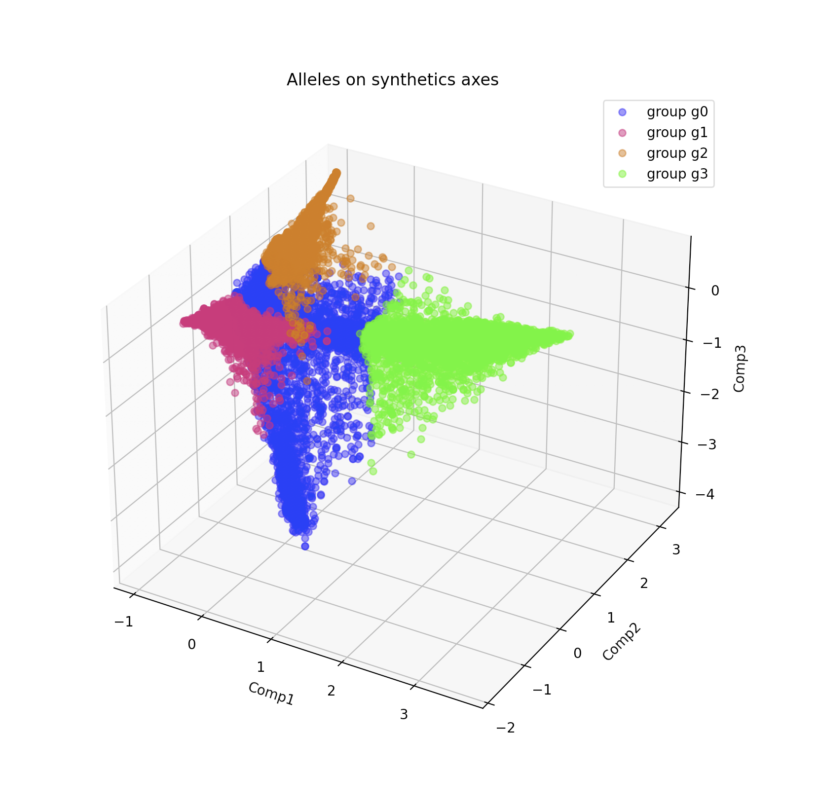
This 3d visualization can be rotated with the mouse.